Pin-hole Model

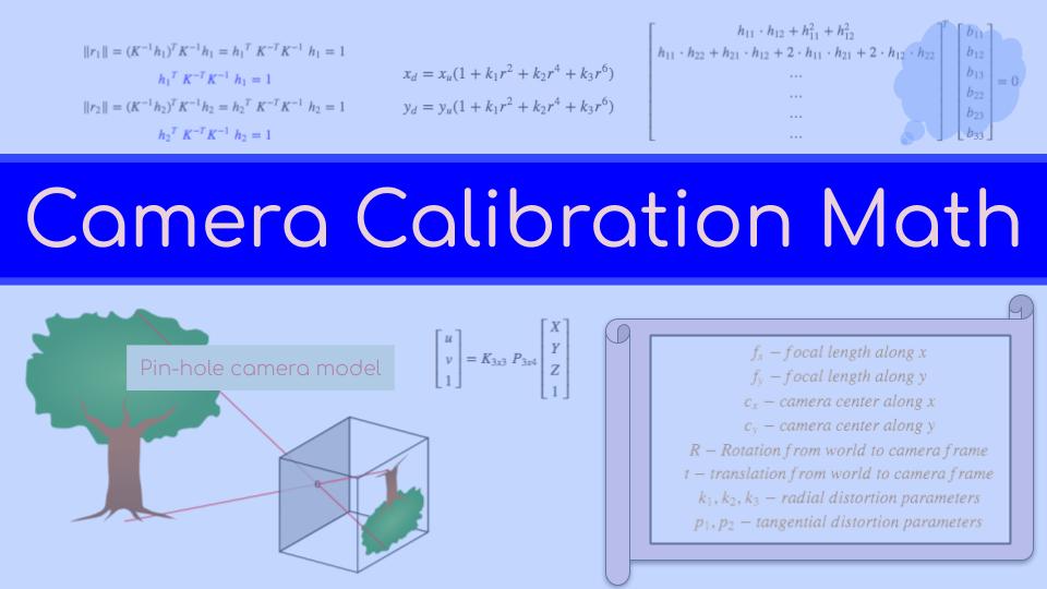
A pin-hole model is the simplest way to explain the working of a camera. Though a real camera is much more sophisticated the underlying principles are the same. Light rays passing through a pin-hole forms an image on the other side. We can use the pin-hole camera as a mathematical model for studying the camera. In fact, most of the math involving camera system are derived using the pin-hole camera model.

The pinhole camera model describes the mathematical relationship between the coordinates of a point in three-dimensional space and its projection onto the image plane of an ideal pinhole camera

It is generally denoted in homogeneous form as, $$\begin{bmatrix} u \\ v \\ 1 \end{bmatrix} = K_{3x3} \begin{bmatrix} R_{3x3} \;| \; t_{3x1} \end{bmatrix} \begin{bmatrix} X \\ Y \\ Z \\ 1 \end{bmatrix}$$

Where $u$ and $v$ are the coordinates on the image and $X$, $Y$ and $Z$ are the 3d coordinates of the point in the world coordinate frame. There are two matrices that handle this transformation, $K$ and $P$. The $K$ matrix is called the intrinsic or camera matrix. This is the matrix that defines the properties of the camera. It is of the form $$K = \begin{bmatrix} f_x & 0 & c_x \\ 0 & f_y & c_y \\ 0 & 0 & 1 \end{bmatrix}$$ where $f_x$ and $f_y$ denote the focal lengths (in pixel units) and $c_x$ and $c_y$ denote the point the principle axis passes through the image plane.

The extrinsic or projection matrix $P$ comprises of the rotation component $R$ and translation component $t$. This matrix transforms the point in the world coordinates to the local camera coordinates.

Inaccuracies and Distortions

In a perfect world this model will sufficiently represent the camera image and we will all be happy. However we are not in a perfect world. The first issue arises because of the pin-hole itself. Since we are talking about a small hole, it only allows a small amount of line to seep in. To make this work, we should either have a high intensity light source or highly sensitive pixels or imaging sensor. In the absence of both we can tackle the problem easily using an optical lens. The lens focusses the light beams to the imaging sensor and thus letting in more light. However the lens can have some imperfections. These imperfections can cause the image to warp and they are called radial distortions.

Barrel (positive radial distortion) and pincushion (negative radial distortion) (courtesy: wikipedia)

The radial distortion can be modelled using non-linear equations of the form, $$x_d = x_u(1 + k_1 r^2 + k_2 r^4 + k_3 r^6)$$ $$y_d = y_u(1 + k_1 r^2 + k_2 r^4 + k_3 r^6)$$ where, $$r = \sqrt{x_u^2 + y_u^2}$$ $x_d$ and $y_d$ are the distorted image coordinates and $x_u$ and $y_u$ are the undistorted image coordinates.

$k_1$, $k_2$ and $k_3$ are the parameters of the radial distortion.

The other problem that comes with the lens is that it has to be mounted parallel to the imaging sensor. It is not an issue in the pin-hole model as there is just a single point in place of the lens. These are called tangential distortions. It is modelled using the following non-linear equations.

$$x_d = x + [2 p_1 x_u y_u + p_2 (r^2 + 2 x^2)]$$ $$y_d = y + [p_1 (r^2 + 2 y_u^2) + 2 p_2 x_u y_u ]$$

$p_1$ and $p_2$ are the parameters of tangential distortion.

Parameters

To model the camera fully, the calibration procedure needs to evaluate the intrinsic, extrinsic and the distortion parameters. Explicitly, these are $$ f_x - focal\ length\ along\ x \\ f_y - focal\ length\ along\ y\\ c_x - camera\ center\ along\ x\\ c_y - camera\ center\ along\ y \\ R_{3x3} - Rotation\ from\ world\ to\ camera\ frame\\t_{3x1} - translation\ from\ world\ to\ camera\ frame\\ k_1, k_2, k_3 - radial\ distortion\ parameters \\ p_1, p_2 - tangential\ distortion\ parameters$$

Procedure

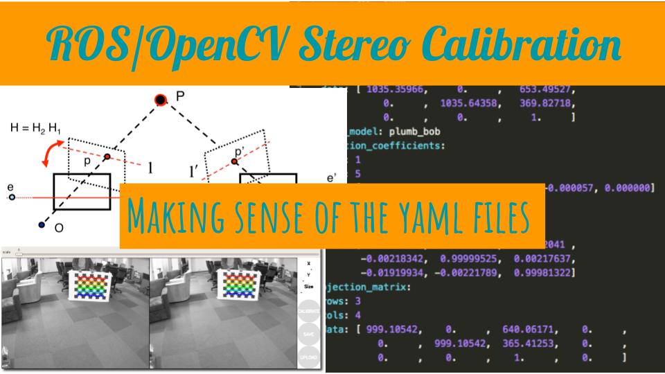
If we know the location of the 3d points and the location of their 2d projections in the image, we can formulate a procedure to estimate these parameters. There are different methods to start with an known set of 3d points. They range from carefully constructed 3d shapes like spheres or cubes to observing points on a plane. The checkerboard method has emerged as a standard where a checkerboard pattern is printed on a planar surface and used for calibration. This method is used mainly because it is easier to identify the checkerboard corners in an image programatically and the pattern can be printed out easily. For the calibration procedure, the checkerboard pattern is placed on a rigid planar surface and it is observed from different orientations and positions. To make the calculations easier we can set the world coordinate frame to align with the checkerboard plane ($XY$ world plane coincides with the checkerboard plane). We can set the origin on one of the checkerboard corners. Since we know the dimensions of the checkerboard square, we can generate the 3d coordinates in the world frame. The pixel coordinates of the checkerboard corners are then observed. Using these two sets of values we can then estimate the parameters as follows.

Math

$$ \require{color} $$

The monocular calibration procedure finds the intrinsic or camera matrix $K$ and the extrinsic or projection matrix $P$ given by the form $$\begin{bmatrix} u \\ v \\ 1 \end{bmatrix} = K_{3x3} \; P_{3x4} \begin{bmatrix} X \\ Y \\ Z \\ 1 \end{bmatrix}$$

Where $X$, $Y$ and $Z$ are the 3d coordinates of a point in the world coordinates and $u$ and $v$ are the pixel coordinates of the same point on the image. The projection matrix transforms the point in the world coordinate to the camera coordinate. The projection matrix comprises of the rotation component $R$ and the translation component $t$.

$$\begin{bmatrix} u \\ v \\ 1 \end{bmatrix} = K_{3x3} \begin{bmatrix} R_{3x3} \;| \; t_{3x1} \end{bmatrix} \begin{bmatrix} X \\ Y \\ Z \\ 1 \end{bmatrix}$$

The intrinsic or camera matrix, $K_{3x3}$ matrix is of the form: $$K = \begin{bmatrix} f_x & 0 & c_x \\ 0 & f_y & c_y \\ 0 & 0 & 1 \end{bmatrix}$$

Expanding,

$$\begin{bmatrix} u \\ v \\ 1 \end{bmatrix} = K_{3x3} \begin{bmatrix} r_{11} & r_{12} & r_{13} & t_1 \\ r_{21} & r_{22} & r_{23} & t_2 \\ r_{31} & r_{32} & r_{33} & t_3 \end{bmatrix} \begin{bmatrix} X \\ Y \\ Z \\ 1 \end{bmatrix}$$

$$\begin{bmatrix} u \\ v \\ 1 \end{bmatrix} = K_{3x3} \begin{bmatrix} X \cdot r_{11} & Y \cdot r_{12} & Z \cdot r_{13} & t_1 \\ X \cdot r_{21} & Y \cdot r_{22} & Z \cdot r_{23} & t_2 \\ X \cdot r_{31} & Y \cdot r_{32} & Z \cdot r_{33} & t_3 \end{bmatrix} $$

As mentioned in the procedure, we set the world coordinate origin on the checkerboard and assume that the checkerboard plane aligns with the $XY$ world plane. This means all the points (including the corner points) on the checkerboard will have $Z=0$ (as its in the $XY$ plane). Therefore the third column is all zeros (marked in red).

$$\begin{bmatrix} u \\ v \\ 1 \end{bmatrix} = K_{3x3} \begin{bmatrix} X \cdot r_{11} & Y \cdot r_{12} & \color{red}{Z \cdot r_{13}} & t_1 \\ X \cdot r_{21} & Y \cdot r_{22} & \color{red}{Z \cdot r_{23}} & t_2 \\ X \cdot r_{31} & Y \cdot r_{32} & \color{red}{Z \cdot r_{33}} & t_3 \end{bmatrix} $$

We can rewrite the same ignoring the third column in the rotation matrix as $$\begin{bmatrix} u \\ v \\ 1 \end{bmatrix} = K_{3x3} \begin{bmatrix} r_{11} & r_{12} & t_1 \\ r_{21} & r_{22} & t_2 \\ r_{31} & r_{32} & t_3 \end{bmatrix} \begin{bmatrix} X \\ Y \\ 1 \end{bmatrix}$$

$$\begin{bmatrix} u \\ v \\ 1 \end{bmatrix} = K_{3x3}\; P_{3x3} \begin{bmatrix} X \\ Y \\ 1 \end{bmatrix}$$

$K_{3x3}\; P_{3x3} = H$ is a $3x3$ matrix which can be treated as a homography as it maps the points in the checkerboard plane to the image plane.

$$\begin{bmatrix} u \\ v \\ 1 \end{bmatrix} = H_{3x3} \begin{bmatrix} X \\ Y \\ 1 \end{bmatrix}$$

Since we know the size of the boxes in the checkerboard (in metric units) we can calculate the $X$ and $Y$ values. Similarly we can find the pixel coordinates, $u$ and $v$ from the images. From these sets of values we should be able to calculate the homography H. Given that we know H, we need to find the camera matrix $K_{3x3}$ and the projection matrix $P_{3x3}$. However the camera matrix, $K$ and the projection matrix $P$ are not arbitary. They have a specific structure.

$K$ is of the form $\begin{bmatrix} f_x & 0 & c_x \\ 0 & f_y & c_y \\ 0 & 0 & 1 \end{bmatrix}$ (upper triangular) and the first two columns of $P$ are from a rotation matrix. Hence they are orthgonal and their magnitude should be 1. We will use these properties to constrain the system and solve for these matrices.

$$ H = K_{3x3} \; P_{3x3}$$

$$ \begin{bmatrix} h_1 & h_2 & h_3 \end{bmatrix} = K \; \begin{bmatrix} r_1 & r_2 & t\end{bmatrix}$$

Now premultiplying with $K^{-1}$ we get, $$ K^{-1} \begin{bmatrix} h_1 & h_2 & h_3 \end{bmatrix} = \begin{bmatrix} r_1 & r_2 & t\end{bmatrix}$$ Where $h_1$, $h_2$ and $h_3$ are the columns of $H$ and $r_1$, $r_2$ and $t$ are the columns of $P_{3x3}$.

$$\color{blue}{\begin{equation} K^{-1} h_1 = r_1 \;\;\; \; \; K^{-1} h_2 = r_2 \; \; \; \; \; K^{-1} h_3 = t \label{eqn:decompose_h} \end{equation}}$$

As I mentioned before, $r_1$ and $r_2$ form the orthonormal basis and hence their norm is 1 i.e., $\left\lVert r_1 \right\rVert = 1$ and $\left\lVert r_2 \right\rVert =1$ and their dot product is zero i.e., $r_1^Tr_2 = 0$. We are going to use these two constraints to solve this equation.

$$r_1^Tr_2 = 0 = {\left(K^{-1} h_1\right)}^T \; K^{-1} h_2 = h_1^T \; K^{-T} K^{-1} \; h_2 $$

$$ \begin{equation} \color{blue}{h_1^T \; K^{-T} K^{-1} \; h_2 = 0} \label{eqn:dotprod} \end{equation} $$

Now considering the norm, $$\left\lVert r_1 \right\rVert = (K^{-1} h_1)^T K^{-1} h_1 = {h_1}^T \; K^{-T} K^{-1} \; h_1 = 1 $$

$$ \begin{equation} \color{blue}{{h_1}^T \; K^{-T} K^{-1} \; h_1 = 1 } \label{eqn:norm1} \end{equation} $$

$$\left\lVert r_2 \right\rVert = (K^{-1} h_2)^T K^{-1} h_2 = {h_2}^T \; K^{-T} K^{-1} \; h_2 = 1 $$

$$ \begin{equation} \color{blue}{{h_2}^T \; K^{-T} K^{-1} \; h_2 = 1} \label{eqn:norm2} \end{equation} $$

The upper triangular nature of $K$ makes $K^{-T} K^{-1}$ a symmetric and positive definite matrix. $$B = K^{-T} K^{-1} = \begin{bmatrix} b_{11} & b_{12} & b_{13} \\ \color{red}{b_{12}} & b_{22} & b_{23} \\ \color{red}{b_{13}} & \color{red}{b_{23}} & b_{33} \end{bmatrix}$$

Substituting and expanding equation $\ref{eqn:dotprod}$ we get, $$ \begin{bmatrix} h_{11} \\ h_{21} \\ h_{31} \end{bmatrix}^T \begin{bmatrix} b_{11} & b_{12} & b_{13} \\ b_{12} & b_{22} & b_{23} \\ b_{13} & b_{23} & b_{33} \end{bmatrix} \begin{bmatrix} h_{12} \\ h_{22} \\ h_{32} \end{bmatrix} = 0 $$

$$ \begin{bmatrix} h_{11} & h_{21} & h_{31} \end{bmatrix} \begin{bmatrix} b_{11} \cdot h_{12} + b_{12} \cdot h_{22} + b_{13} \cdot h_{32} \\ b_{12} \cdot h_{12} + b_{22} \cdot h_{22} + b_{23} \cdot h_{32} \\ b_{13} \cdot h_{12} + b_{23} \cdot h_{22} + b_{33} \cdot h_{32} \end{bmatrix} = 0 $$

$$\begin{equation} h_{11} \cdot b_{11} \cdot h_{12} + h_{11} \cdot b_{12} \cdot h_{22} + h_{11} \cdot b_{13} \cdot h_{32} + \\ h_{21} \cdot b_{12} \cdot h_{12} + h_{21} \cdot b_{22} \cdot h_{22} + h_{21} \cdot b_{23} \cdot h_{32} + \\ h_{31} \cdot b_{13} \cdot h_{12} + h_{31} \cdot b_{23} \cdot h_{22} + h_{31} \cdot b_{33} \cdot h_{32} = 0 \label{eqn:prod_expanded} \end{equation}$$

Similarly substituting and expanding equation $\ref{eqn:norm1}$ and equation $\ref{eqn:norm2}$ we get equation $\ref{eqn:norm1_expanded}$ and equation $\ref{eqn:norm2_expanded}$ respectively.

$$\begin{equation} h_{11}^2 \cdot b_{11} + h_{11} \cdot b_{12} \cdot h_{21} + h_{11} \cdot b_{13} \cdot h_{31} + \\ h_{21} \cdot b_{12} \cdot h_{11} + h_{21}^2 \cdot b_{22} + h_{21} \cdot b_{23} \cdot h_{31} + \\ h_{31} \cdot b_{13} \cdot h_{11} + h_{31} \cdot b_{23} \cdot h_{21} + h_{31}^2 \cdot b_{33} = 0 \label{eqn:norm1_expanded} \end{equation}$$

$$\begin{equation} b_{11} \cdot h_{12}^2 + h_{12} \cdot b_{12} \cdot h_{22} + h_{12} \cdot b_{13} \cdot h_{32} + \\ h_{22} \cdot b_{12} \cdot h_{12} + b_{22} \cdot h_{22}^2 + h_{22} \cdot b_{23} \cdot h_{32} + \\ h_{32} \cdot b_{13} \cdot h_{12} + h_{32} \cdot b_{23} \cdot h_{22} + b_{33} \cdot h_{32}^2 = 0 \label{eqn:norm2_expanded} \end{equation}$$

Rearranging,

$${\begin{bmatrix} h_{11} \cdot h_{12} +h_{11}^2 + h_{12}^2 \\ h_{11} \cdot h_{22} + h_{21} \cdot h_{12} + 2 \cdot h_{11} \cdot h_{21} + 2 \cdot h_{12} \cdot h_{22} \\ … \\ … \\ … \\ … \end{bmatrix}}^T \; \begin{bmatrix} b_{11} \\ b_{12} \\ b_{13} \\ b_{22} \\ b_{23} \\ b_{33} \end{bmatrix} = 0 $$

Solving the above equation for $b_{11} … b_{33}$ yields the $B$ matrix. We can then apply Cholesky decomposition on $B$. Since $B$ is symmetric we get $B = LL^T$ where $L = K^{-T}$.

Substituting $K^{-1}$ in equation $\ref{eqn:decompose_h}$ we can get $t$.

Thus we recover the intrinsics or camera matrix, $K$ and the extrinsics or projection matrix, $P$ using the checkerboard calibration procedure.

The distortion parameters are estimated using a non-linear optimization technique like Levenberg Marquardt. I will expand on this in a later post.

References

• The slides from Barbara Frank, et.al., is very helpful in understanding the math.
• The OpenCV camera calibration tutorial is helpful if you are interested in implementing this using OpenCV.