For those of you who have done stereo calibration in the past (a few years ago), will remember it was not easy. Then came the famous camera calibration toolbox for Matlab developed by Bouguet. It made things a lot easier. Then OpenCV implemented these methods in C++ and that added even more control. ROS took it the next level and made the calibration process a lot easier and interactive. I really like the feature where they tell you in which way you need to move the calibration target to get a better calibration.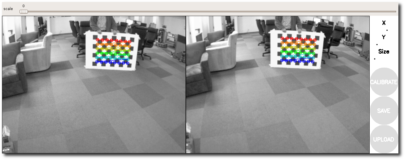

After you run the calibration procedure, the program creates a tar ball of all the calibration images and the right and left camera yaml files (stores it as /tmp/calibrationdata.tar.gz). A typical yaml file for the left camera will look something like this:

 1
 2
 3
 4
 5
 6
 7
 8
 9
10
11
12
13
14
15
16
17
18
19
20
21
22
23
24
25
26

image_width: 1280
image_height: 720
camera_name: stereo/left
camera_matrix:
  rows: 3
  cols: 3
  data: [ 1035.35966,     0.     ,   653.49527,
             0.     ,  1035.64358,   369.82718,
             0.     ,     0.     ,     1.     ]
camera_model: plumb_bob
distortion_coefficients:
  rows: 1
  cols: 5
  data: [-0.337964, 0.123943, -0.000500, -0.000057, 0.000000]
rectification_matrix:
  rows: 3
  cols: 3
  data: [ 0.99981329,  0.00214123,  0.0192041 ,
         -0.00218342,  0.99999525,  0.00217637,
         -0.01919934, -0.00221789,  0.99981322]
projection_matrix:
  rows: 3
  cols: 4
  data: [ 999.10542,    0.     ,  640.06171,    0.     ,
            0.     ,  999.10542,  365.41253,    0.     ,
            0.     ,    0.     ,    1.     ,    0.     ]

Image Dimensions

Lines 1 and 2 specify the image width and height. An interesting fact is, you can resize the image and use the same calibration values. The only thing you will need to scale accordingly is the camera matrix ($K$). The same distortion parameters just work.

Camera Matrix, $K$

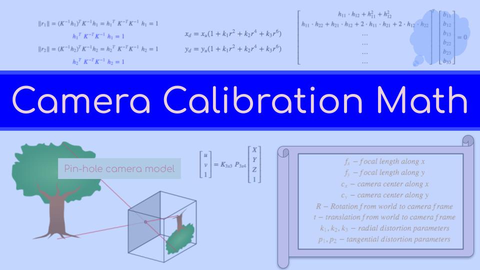
The camera matrix is typically represented as $K$. This is also called the intrinsic matrix. It is an upper triangular matrix of the form $$K = \begin{bmatrix} f_x & skew & c_x \\ 0 & f_y & c_y \\ 0 & 0 & 1 \end{bmatrix}$$ where $f_x$ and $f_y$ are the focal lengths along the $X$ and $Y$ axes, $c_x$ and $c_y$ are the camera centers and $skew$ is the skew factor which is almost always zero. An important point to note here is that the focal length is in the pixel units. It is not in any metric dimensions. Generally the $f_x$ and $f_y$ values are pretty similar for a good quality camera. This just means that the pixels are squares. These values will be different if the pixels are rectangles ie., the horizontal size of a pixel is different from its vertical size. If the pixel is parallelogram instead of a square or rectangle, then we will see the skew factor coming into effect.

Distortion Parameters, $D$

As you may already know, an ideal pin-hole camera will have zero distortion. But it is not true for a real camera. You can think of the distortion parameters as a mathematical way of explaining away the inaccuracies in the image. Distortions are mathematical models which can express the manufacturing inaccuracies of the cameras and lenses. There are different models we could use to explain the inaccuracies. Plumb Bob is the most famous distortion model (introduced by Brown in 1966) that is implemented in OpenCV. There are two types of distortions. The first one is called radial distortion which is caused by the lens. The distortion is the constant at a given distance from the principle point. It looks something like this (fish-eye effect).

Barrel and pincushion distortions (courtesy: wikipedia)

The radial distortion can be explained using three parameters and can be explained using the following equation. $$x_{distorted} = x(1 + k_1 r^2 + k_2 r^4 + k_3 r^6)$$ $$y_{distorted} = y(1 + k_1 r^2 + k_2 r^4 + k_3 r^6)$$ where, $$r = \sqrt{(x - c_x)^2 + (y - c_y)^2} $$

$c_x$ and $c_y$ are the camera centers from the camera matrix, $K$. For more details on these equations refer to this page or Brown’s[1] paper.

The second type of distortion is caused due to inaccuracies in the mounting of the camera sensor such that it does not align to the center. This causes the imaging plane to not be parallel to the lens. This distortion can be explained using two parameters $p_1$ and $p_2$.

$$x_{distorted} = x + [2 p_1 x y + p_2 (r^2 + 2 x^2)]$$ $$y_{distorted} = y + [p_1 (r^2 + 2 y^2) + 2 p_2 x y ]$$

Typically for high-end cameras where care is taken in the sensor mounting process, these parameters are pretty small. For cheap consumer grade cameras which are mass produced, these parameters could be high. However, nowadays with increase in efficiencies in manufacturing processes, these values are smaller even for cheaper cameras.

Similarly the radial distortion parameters could be high for cheap plastic lenses and typically low for high-end glass lenses.

It has to be noted that these five parameters will not be able to explain every inaccuracy in the image. If the lens or camera sensor have serious manufacturing issues, it is possible that even after estimating decent values for these parameters, the image might still look distorted. Also keep in mind that these parameters are estimated using non-linear optimization techniques like Levenberg Marquardt. The final solution is sensitive to initial conditions. Severe distortions could lead to local minima. We could think of using even more parameters to explain the inaccuracies, but at that point, the non-linear effects will dominate and obtaining a global minima will become impossible.

Rectification Matrix, $R_{rect}$

This is the matrix which helps the stereo depth estimation algorithm to quickly estimate the depth of each pixel in the image. As a refresher lets look at how stereo matching happens. From epipolar geometry, for every pixel in one image there is a line called epipolar line that we have to search for correspondence in the other image. We will cover epipolar geometry in a different article. The image below shows how epipolar geometry is used to find correspondences.

Using epipolar geometry to find correspondences (courtesy: wikipedia)

The epipolar line search becomes a lot faster if the epipolar lines are aligned to the pixel rows. This is what the rectification matrix does. It reprojects the camera images so that the epipolar planes are parallel. The figure belows shows this process. You will see that the epipolar lines become parallel (epipoles are at infinity). Now for every pixel in the left image, you just have to search for the corresponding pixel in the same row.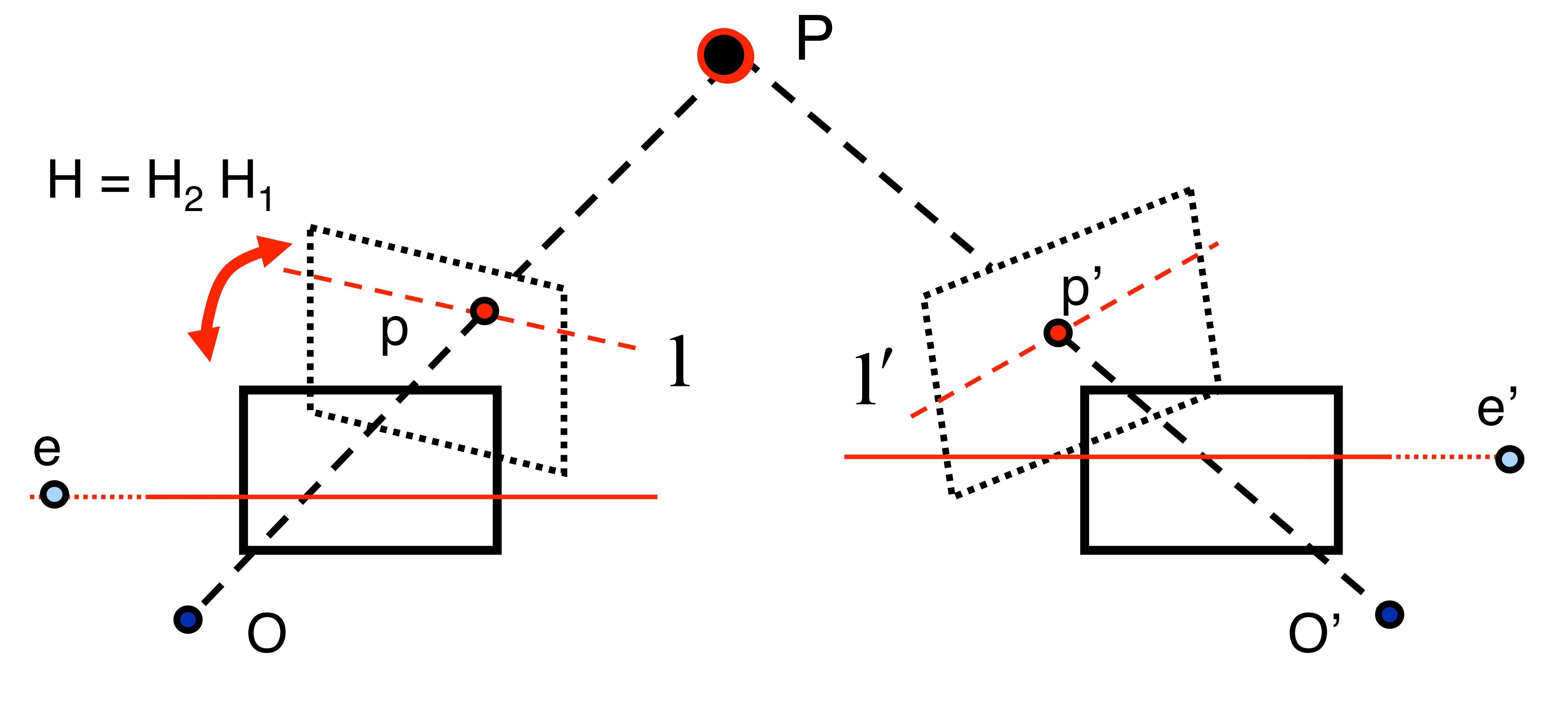

Projection Matrix, $P$

We have to be careful that this is not the regular projection matrix used in computer vision literature. It has a similar form though. I got tripped by this several times in the past. In fact that is the motivation for me to write this article. If this is not the regular projection matrix what is it then?

$$ \begin{bmatrix} u \\ v \\ 1 \end{bmatrix} = K * [R | t] * \begin{bmatrix} X \\ Y \\ Z \\ 1 \end{bmatrix}$$

This is the regular camera projection equation. It projects a 3D point to 2D image. Here $\begin{bmatrix}u & v & 1\end{bmatrix}^T$ is the homogenous pixel coordinates. $K$ is the intrinsic camera matrix which we saw before, $\begin{bmatrix} X & Y & Z & 1 \end{bmatrix}^T$ is the homogeneous 3D point in the world coordinate frame. $[R | t]$ is the projection matrix which projects the 3D from the world coordinates to the camera coordinate frame.

However the projection matrix that we have here is different. For the left camera it is of the form: $$ P^l = \begin{bmatrix} f & 0 & c_x & 0 \\ 0 & f & c_y & 0 \\ 0 & 0 & 1 & 0 \end{bmatrix} $$ and for the right camera it is of the form: $$ P^r = \begin{bmatrix} f & 0 & c_x & T_x * f \\ 0 & f & c_y & 0 \\ 0 & 0 & 1 & 0 \end{bmatrix} $$

The first 3x3 elements correspond to the camera matrix $K$ after the rectification. The last column will be all zeros for the left camera or for monocular cameras. For horizontal stereo setup (that is the left-right camera setup) the first entry will be $T_x * f$ and and the rest are all zeros.

For vertical stereo setup (top down setup) the second entry will be $T_y * f$ and the rest are all zeros. It will be of the form: $$ P^d = \begin{bmatrix} f & 0 & c_x & 0\\ 0 & f & c_y & T_y * f \\ 0 & 0 & 1 & 0 \end{bmatrix} $$

Here is a sample of the right camera yaml file.

21
22
23
24
25
26

projection_matrix:
  rows: 3
  cols: 4
  data: [ 999.10542,    0.     ,  640.06171,  -79.98422,
            0.     ,  999.10542,  365.41253,    0.     ,
            0.     ,    0.     ,    1.     ,    0.     ]

Note that this equation does not have the camera matrix $K$ which is sucked into the projection matrix $P$. We don’t need the rotation and translations because we are using the rectified image which already accounts for those. If you want to extract the baseline between the cameras, use this formula.

$$ baseline = \frac{-T_x}{f}$$

The units will be whatever units you used to measure the length of the checkerboard squares during calibration.

References

[1]: Close-Range Camera Calibration, D.C. Brown, Photogrammetric Engineering, pages 855-866, Vol. 37, No. 8, 1971.