The famous filtering algorithms like Kalman filter (KF), Extended KF and particle filter (PF) are all derivatives of Bayes filter. They either use gaussian distributions (think KF) or approximations of it (think EKF) or multimodal distributions (think PF) to represent the posterior. But essentially they are all Bayes filter in essence.

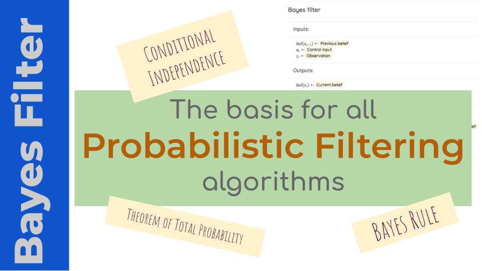
The Bayes filter is an algorithm that incorporates observations and control inputs to a system to form a belief (posterior) using the Bayes rule. The general algorithm looks like this

This is the generic structure of Bayes filter which is shared by other filters like PF and EKF as well. Once this structure is understood, it should be easy to understand what each of the filters do in specific. This is the underlying framework.

Let us now try to break it down and understand each of the components in the Bayes filter and define them rigourously.

Let $X$ represent the state of the system. This can be a single random variable or a list of them in a vector. It could represent anything in the world that we are trying to estimate using the probabilistic framework. For example, it can represent the position of a robot (in 2D) using three random variables $x, y, \theta$.

The state at time $t$ is given by $X_t$.

The belief is just a probability distribution of the state we are interesed in at any time $t$. That is, $$bel(X_t) = P(X_t)$$ Therefore, the belief at the previous time step is $bel(X_{t-1})$ and current belief is $bel(X_t)$.

The control input is the action we performed on the system with the intension to change the state of the system. For example, this could be spinning the wheels to change the position of the robot. The control input is usually represented as $u_t$.

Observation is what the sensors measures looking at the environment. For example, this could be an encoder reading from our robot’s wheels or feedback from the camera systems stating how much we moved. Observations are usually represented as $z_t$.

The Bayes filter algorithm can be rewritten as:

If you notice carefully, you will see that I have just redefined item in the pseudocode with proper mathematical terms. As I mentioned before, this is the basic framework for any filtering algorithm.

Derivation

Let us now go through the derivation. At first look, it will appear daunting. But if you follow it closely, there are only a few basic rules we use to arrive at the solution. We need to prove that the posterior distribution $p(x_t | z_{1:t}, u_{1:t})$ (probability of the current state given all the previous measurements and control inputs) is calculated correctly from the previous posterior distribution $p(x_{t-1} | z_{1:t-1}, u_{1:t-1})$. We will prove this using mathematical induction.

Before we delve into the derivation we will first revisit two main rules we will use here.

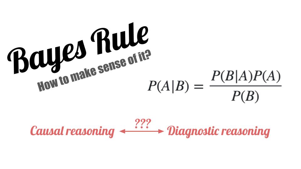
Bayes Rule

Ofcourse, we will use Bayes rule. It is stated as $$p(a|b) = \frac{p(b|a) . p(a)}{p(b)}$$ To get a deeper understanding and the underlying intution refer to the Bayes rule article.

Conditional Independence

If $x$, $y$ and $z$ are three random variables and if $y$ carries no information about $x$ if $z$ is known, then through conditional independence we get, $$p(x|z) = p(x|z,y)$$

Theorem of Total Probability

Theorem of total probability follows from conditional probabilities. It is used for marginalizing variables. If $x$ and $y$ are independent variables, then the total probability is given by:

$$p(x) = \int { p(x|y) p(y) dy}$$

Take a look at this video for indepth understanding of this law.

Proof

We need to prove that the probability of the state at the current time step follows from probability of the previous time step given all the measurements and control inputs. Let us start with the probability of the current time step $bel(x_t) = p(x_t | z_{1:t}, u_{1:t})$. It can be rewritten as, $$p(x_t | z_{1:t}, u_{1:t}) = p(x_t | z_t, z_{1:t-1}, u_{1:t}) $$ Now applying Bayes rule, $$bel(x_t) = p(x_t | z_{1:t}, u_{1:t}) = \frac{p(z_t | x_t, z_{1:t-1}, u_{1:t}) \;\;p(x_t|z_{1:t-1},u_{1:t})}{p(z_{1:t-1},u_{1:t})} $$

As I mentioned in the Bayes rule article, the denominator is just a normalizing term which can be replaced with $\eta$. Therefore $$bel(x_t) = p(x_t | z_{1:t}, u_{1:t}) = \eta p(z_t | x_t, z_{1:t-1}, u_{1:t}) \;p(x_t|z_{1:t-1},u_{1:t}) $$

Since the current measurement $z_t$ does not depend on the previous measurements or control inputs due to conditional independence, the first term becomes, $$p(z_t | x_t, z_{1:t-1}, u_{1:t}) = p(z_t | x_t)$$

Therefore the posterior becomes, $$bel(x_t) = p(x_t | z_{1:t}, u_{1:t}) = \eta \; p(z_t | x_t) \;p(x_t|z_{1:t-1},u_{1:t}) $$

If we call the second term $\bar{bel}(x_t)$ ie., belief before incorporating the measurement we get, $$bel(x_t) = \eta \; p(z_t | x_t) \; \bar{bel}(x_t)$$

This is exactly the line in our algorithm which incorporates the observation and its called the sensor model.

Let us now expand $\bar{bel}(x_t)$. $$ \bar{bel}(x_t) = p(x_t|z_{1:t-1},u_{1:t}) $$

Using the theorem of total probability we introduce the previous state $x_{t-1}$, $$ \bar{bel}(x_t) = \int{p(x_t|x_{t-1},z_{1:t-1},u_{1:t}) \; p(x_{t-1} | z_{1:t-1}, u_{1:t}) \; dx_{t-1}} $$

The current state $x_t$ and the previous state $x_{t-1}$ are conditionally independent of the previous measurements and control inputs (except the control input at the current step) $$ p(x_t|x_{t-1},z_{1:t-1},u_{1:t}) = p(x_t| x_{t-1}, u_t)$$

However for the second term which is the probability of the previous state, it is not impacted but the control input at the current time step. Therefore the second term becomes, $$p(x_{t-1} | z_{1:t-1}, u_{1:t}) = p(x_{t-1} | z_{1:t-1}, u_{1:t-1})$$

Using these two results in the previous belief, we get, $$ \bar{bel}(x_t) = \int{ p(x_t| x_{t-1}, u_t) \; p(x_{t-1} | z_{1:t-1}, u_{1:t-1}) dt } $$

This is the line in the algorithm which incorporates the control input into the belief. If you take a second look, you will notice the second term is actually the belief at the previous time step. Thus we have proved that the current belief derives from the previous belief.

For a concreate implementation we need to know the actual probabilities densities for the measurements $p(z_t|x_t)$, transitions $p(x_t|u_t,x_{t-1})$ and the initial belief $p(x_0)$ which we will obtain when we implement the filter like Kalman filter or particle filter.

Reference

Most of the derivation is taken from Probabilistic Robotics by Sebastian Thrun, Wolfram Burgard and Dieter Fox, Page 31-33