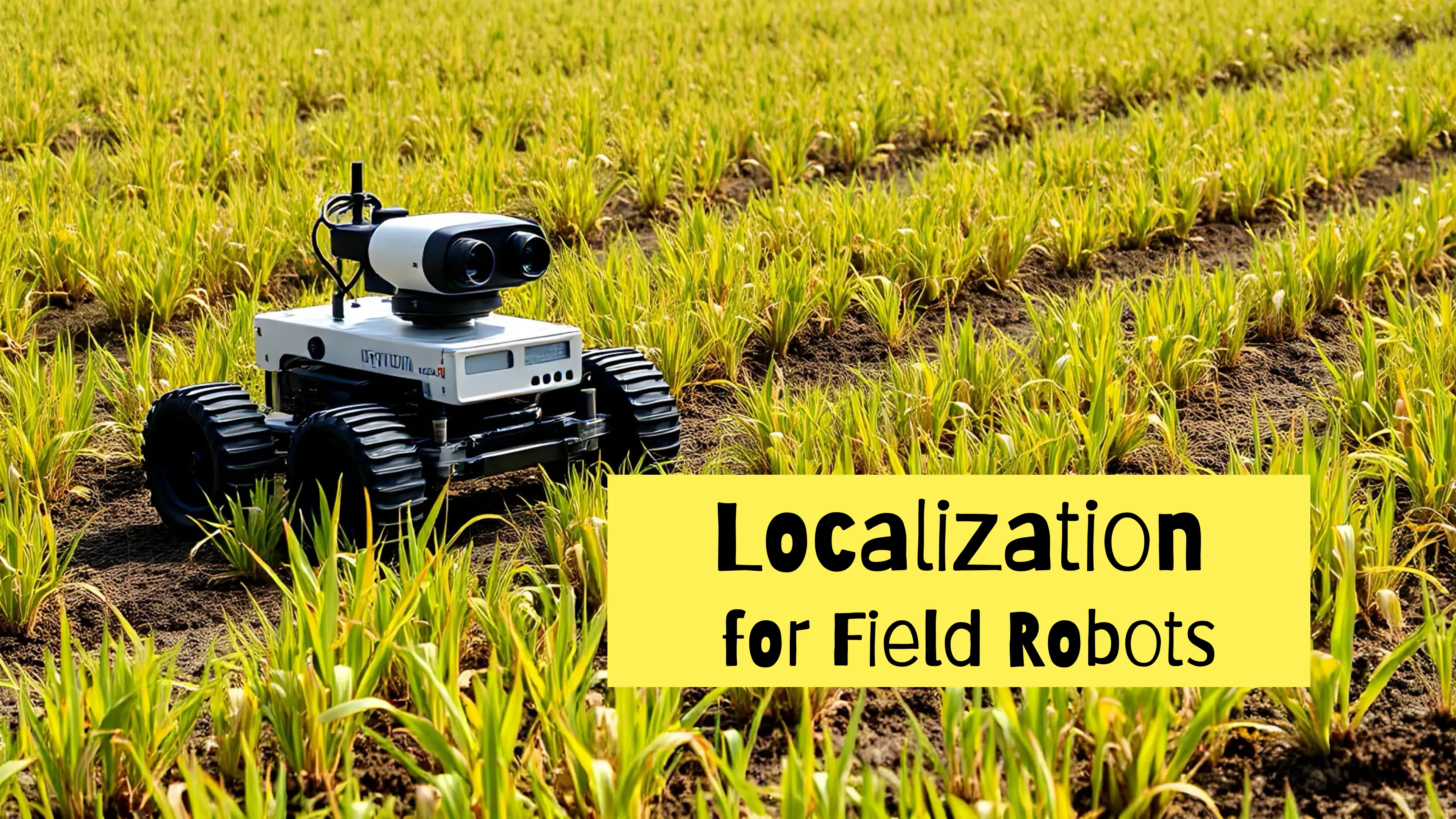
Localization for Field Robots: Navigating the Unstructured World

Field robots—operating outdoors in settings like agriculture, mining, and disaster response—need to determine their position and orientation accurately to perform tasks and avoid obstacles. This process is known as localization, which uses state estimation techniques to predict the robot’s position by combining motion data and sensor measurements. However, localization for field robots is challenging because they operate in unstructured environments, such as forests, uneven terrain, and areas with poor GPS coverage.

This post introduces the key localization techniques, starting with the Bayes filter and how it leads to more advanced methods like the Kalman filter and Extended Kalman Filter (EKF). We’ll also cover particle filters and how they handle uncertainty differently from Kalman-based filters.

1. The Bayes Filter: A Foundation for State Estimation

The Bayes filter provides the basic framework for localization. It uses probabilities to estimate the robot’s position, called its state, by continuously updating a belief based on prior information, control input (e.g., movement commands), and new sensor measurements.

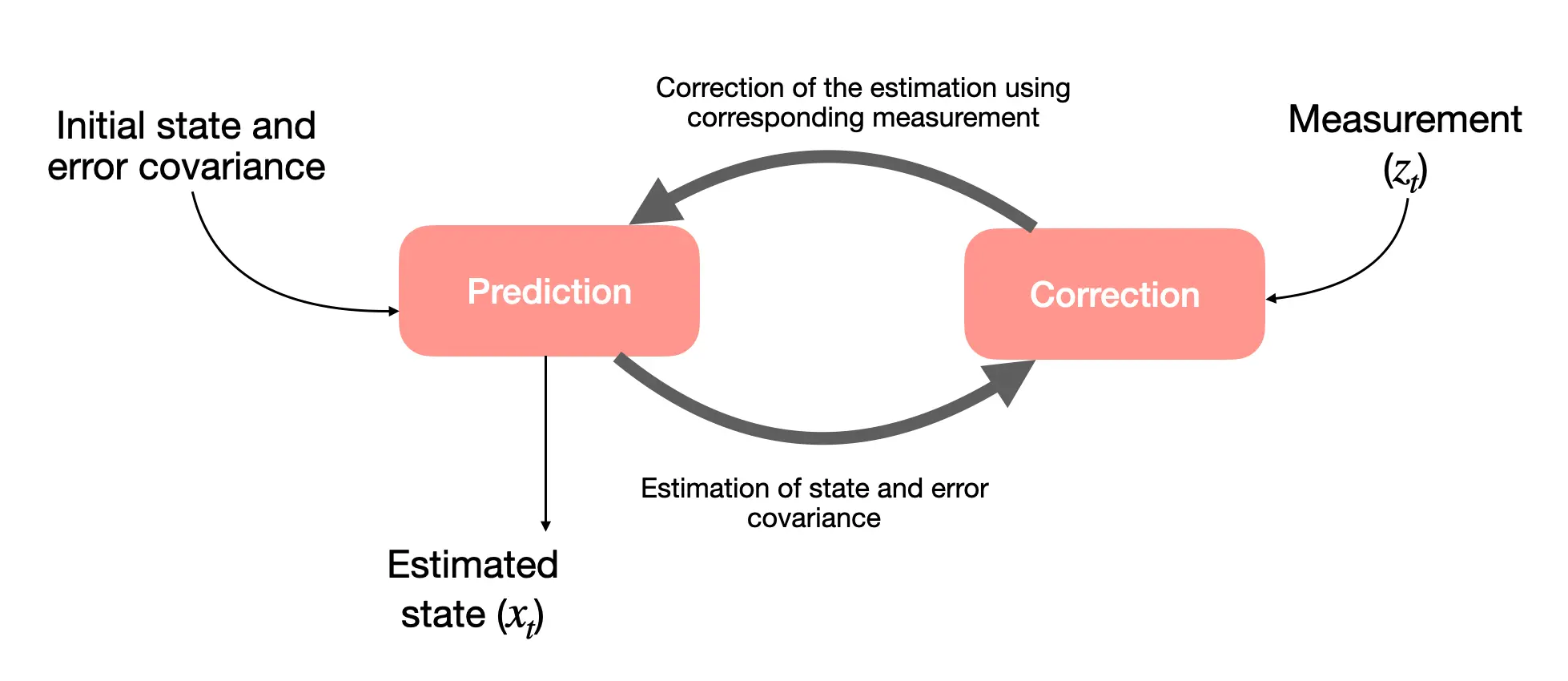
Bayes filters work in two steps:

1. Prediction: Estimate the robot’s next state based on the previous state and control input (e.g., “Move forward 1 meter”).
2. Correction: Use sensor measurements (like LiDAR or GPS) to correct the prediction and reduce errors.

Bayes Filter Formula (Simplified):

$Bel(x_t) = \eta \cdot p(z_t | x_t) \cdot Bel(x_{t-1})$

• $Bel(x_t)$: The belief about the robot’s state at time $t$.
• $p(z_t | x_t)$: Probability of the measurement $z_t$​ given the state $x_t$​.
• $\eta$: A normalization factor to ensure the probabilities sum to 1.

While the Bayes filter provides the theoretical foundation for localization, it can be computationally expensive. To make the process more efficient, we use Kalman filters for systems with linear dynamics. ![[Localization-state-estimation-20241016111106512.webp]] Prediction and correction steps in the Bayes filter

2. The Kalman Filter: Efficient State Estimation for Linear Systems

The Kalman filter (KF) is a fast and efficient method built on the Bayes filter. It assumes that the system dynamics and measurement models are linear, and the noise in the system follows a Gaussian (normal) distribution.

A Kalman filter works in two steps, just like the Bayes filter:

1. Prediction: Estimate the new state and uncertainty based on the previous state and control inputs.
2. Correction: Use sensor data to correct the estimate and improve the accuracy.

Simplified Kalman Filter Equations:

Prediction:

$$\hat{x}_t = $$

$$A \cdot \hat{x}_{t-1} + B \cdot u_t$$

Here:

• $\hat{x}_t$​: Predicted state at time $t$.
• $A$: System dynamics matrix (how the robot’s state evolves).
• $u_t$​: Control input (e.g., wheel speed).
• $B$: Control matrix (how inputs affect the state).

Correction:

$\hat{x}_t = \hat{x}_t + K_t \cdot (z_t - H \cdot \hat{x}_t)$

Here:

• $z_t$​: Sensor measurement at time $t$.
• $H$: Measurement matrix (maps the state to the measurement).
• $K_t$​: Kalman gain, which decides how much to trust the sensor data versus the prediction.

The Kalman filter is useful for systems where the robot’s motion is predictable and linear, like indoor environments. However, field robots often encounter nonlinear dynamics, such as moving over uneven terrain or turning at angles, where Kalman filters struggle. This leads us to the Extended Kalman Filter (EKF).

3. Extended Kalman Filter (EKF): Handling Nonlinear Motion

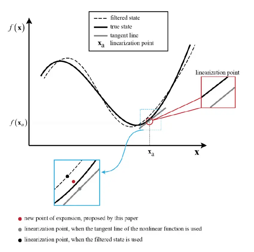
In the real world, robots often encounter nonlinear dynamics. For example, the relationship between the robot’s steering angle and its position can’t always be described with simple linear equations. The Extended Kalman Filter (EKF) extends the Kalman filter to handle nonlinear motion models by using mathematical approximations.

Instead of applying linear equations directly, the EKF:

1. Predicts the next state using nonlinear functions (e.g., trigonometric functions for rotation).
2. Linearizes these functions around the current estimate using a Jacobian matrix, which provides a locally linear approximation.

This allows the EKF to perform well in nonlinear systems, making it suitable for field robots navigating complex terrains. However, the EKF still assumes the noise is Gaussian, which can be a limitation in highly dynamic environments.

4. Particle Filters: Handling Complex and Uncertain Environments

The Particle Filter (PF) offers an alternative approach when the system is highly nonlinear or when the noise is non-Gaussian. Unlike Kalman-based filters that rely on a single state estimate, particle filters use many particles, each representing a possible state of the robot.

Each particle is a hypothesis about the robot’s position. The particles are:

1. Predicted using control inputs to move forward, like the robot would in reality.
2. Weighted based on how well they match the sensor measurements.
3. Resampled so that the most likely particles are kept for the next iteration.

This method is especially useful for environments where the robot might encounter multiple possibilities (e.g., when landmarks are ambiguous, or GPS data is noisy). However, particle filters are computationally expensive because they require many particles to maintain accuracy.

Why Use Particle Filters?

• Advantages:
  • Handles non-Gaussian noise and complex, nonlinear systems.
  • Can represent multi-modal distributions (multiple possible positions).
• Disadvantages:
  • Requires more computation than Kalman-based filters.
  • Slower to run in real-time, especially with many particles.

Conclusion: Choosing the Right Filter for Localization

Localization is critical for field robots to perform tasks effectively, but it presents unique challenges due to unstructured environments and nonlinear dynamics.

• Kalman filters work well when the environment is predictable and the system is mostly linear, such as in indoor applications.
• Extended Kalman filters improve on Kalman filters by handling nonlinearities, making them more suitable for outdoor navigation.
• Particle filters shine in highly dynamic and uncertain environments where noise is non-Gaussian, although they require more computation.

Choosing the right localization algorithm depends on the robot’s environment and the trade-off between accuracy and computational efficiency. As field robotics continues to advance, hybrid approaches that combine multiple filtering techniques will further improve localization, enabling robots to explore and perform tasks autonomously in even more challenging terrains.

Disclosure:
This article includes content generated with the assistance of large language models (LLMs). The generated sections have been reviewed and refined to ensure accuracy and alignment with the topic.